Linux Storage Cache

Linux Content Index

File System Architecture – Part I
File System Architecture– Part II
File System Write
Buffer Cache
Linux File Write 

Every system use case involves a combination of software modules talking to each other. But an optimal system is more than set of efficient modules. The overall architectural arrangement of these modules and their data/control interfaces also impacts the performance. In that sense, several useful design methodologies can be observed from examining the storage sub system within Linux.

Application to VFS
Fig 1

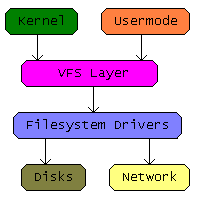
Various abstraction layers have their own purpose. For example, VFS exposes a uniform interface to the user applications, while it’s the file system which actually implements the structural representation of files within the device. Eventually, how each storage sector is accessed will depend on the block driver interactions with the hardware. Productivity depends on how quickly a system can service user requests. In other words, the response time is critical. The pure logic implemented for each of the involved modules could be efficient, but if they are merely stacked up vertically then it will be only as good as using a primitive processor with no internal caches or pipelined executions.

*********************************

Inode-Dentry Cache

Book keeping information associated with each file is represented by two kernel structures — Inodes and Dentries. In bare simple terms these constructs hold the information necessary to identify and locate the storage blocks associated with a file. A multitasking environment might have numerous processes accessing the same volume or even the same file. Caching this information at higher levels can reduce contentions associated with the corresponding lower layers. If the repeated file accesses would be picked from the VFS cache, then the file system will be free to quickly service the new requests. Consider a use case where there are multiple processes looking up for a file in different dedicated directories; without a cache, the contention on the file system will scale with the number of processes. But with a good cache mechanism, only the brand new requests would end up accessing the file system module. The idea is quite like a fully associative hierarchical hardware cache.

Inode/Dentry Cache
Fig 2 – Inode/Dentry Cache

*********************************

Data Cache

Inodes and Dentries are accessed by the kernel to eventually locate the file contents, hence the above cache is only a part of the solution while the data cache handles the rest (see below Fig -3). Even here we need frequently accessed file data to be cached and only the new writes or new reads should end up contending for file system module attention. Please note that inside the kernel, the pages associated with file are arranged as a radix tree indexed via file offsets. While the dentry cache is managed by a hash table. Also, each such data cache is eventually associated with the corresponding Inode.

Cache mechanism also determines the program execution speed, it’s closely related to how efficiently the binary sections of the executable are managed within the RAM. For example, the read-ahead heuristics would determine how often the system endures an executable page miss. Also another useful illustration of the utility of a cache is the use case where a program is accessing files from the same volume where its executable is paging from; without a cache the contention on the file system module would be tremendous.

Full Cache
Fig 3 – Full Cache

*********************************

Cache Management

Cache management involves its own complexities. How these buffers are filled, flushed, invalidated or marked as dirty depends on the file system module. Linux kernel merely invokes the file system registered call-backs and expects that the associated cache buffers would be handled accordingly. For example, during a file overwrite the file system should mark the overwritten cached page as dirty, otherwise the flush may never get invoked for that page.

We can also state that the Linux kernel VFS abstracts the pure logic of how data is represented on the storage device from how it’s viewed by kernel on a running system. In this manner the role of the file system is limited to its core functionality of mapping file access to actual storage blocks and it also deals with the transformation between internal file system specific representation of files to the generic VFS Inode, Dentry and data cache constructs. Eventually, how file is created, deleted or modified and how the associated data cache is managed depends solely on the file system module.

For example, a new file creation would involve invoking of the file system module call-backs registered via kernel structure “inode_operations”. The lookup call-backs registered here would be employed to avoid file name duplication and also the obvious “create inode” call would be needed to create the file. An fopen would invoke “file_operations” callback and similarly a data read/write would involve use of “address_space_operations”.

How the registered file system call-backs would eventually manage the inode, dentry and the page data cache buffers would depend on its own inherent logic. So here there is a kind of loop where the VFS calls the file system module call-backs and those modules would in turn call other kernel helper functions to handle specific cache buffer operations like clean, flush, write-back etc. In the end when the file system call-backs return the control back to VFS the associated caches should be already configured and ready for use.

Inode/Page Cache maps
Fig 4 – Inode/Page Cache maps

*********************************

Load Store Analogy

A generic Linux file system can be described as a module which directly services the kernel cache by implementing functions for creating, invalidating or flushing various cache entries and in this manner it only indirectly caters to the POSIX file operations. The methodology here is in a way analogous to how a RISC load-store would differ from a 8051 like CISC design, separation of the slow memory access from the register operations constitute the core attribute of a load-store mechanism. Here the Linux kernel ensures that the operations on the cache can happen in parallel with an ongoing load or store which might involve the file system and the driver modules, the obvious trade-offs are complexity and memory consumption.

*********************************

Pipelines

Caches are effective when there are read ahead mechanisms and background flusher tasks. A pipelined architecture would involve as much parallel execution as possible. Cache memories are filled in advance by the reader threads while the dirty entries are constantly flushed in the background by worker threads. Such sector I/O requests are asynchronously queued and processed by the block driver task which will eventually DMA them into the interfaced device. After the writes, the corresponding cache entries are marked as clean and similarly after the reads the entries are marked as up-to-date. The pipeline stages can be seen in the below Fig 5.

Kernel Storage Pipeline
Fig 5 – Kernel Storage Pipeline

System organization evolves over time when various use cases are analyzed for performance bottlenecks and the system arrangement itself is constantly revisited to remove those identified issues. Matured generic software architectures adapt effectively to all the intended use cases while remaining  within various resource constraints. For a general purpose operating system like Linux, the infrastructure for cache memory utilization is a good illustration of how various abstract software components can seamlessly coordinate with widely varying user requests.

Linux File System Write

Linux Content Index

File System Architecture – Part I
File System Architecture– Part II
File System Write
Buffer Cache
Storage Cache

Linux file write methodology is specific to particular file systems. For example, JFFS2 will sync data within the user process ‘context’ itself (inside write_end call), while file systems like UBIFS, LogFS, Ext & FAT tends to create dirty pages and let the background flusher task manage the sync.

These two methodologies come with their own advantages, but usage of the second method leads to Linux kernel exhibiting certain quirks which might drastically impact the write throughput measurements.

Linux File Write

The above diagram does give an overview of the design, there are in fact two main attributes to this architecture:

COPY : User space data is copied into a kernel page associated with the file and marked as dirty via“write_begin” and “write_end” file system call backs, they are in fact invoked for every “write” system call made by the user process. So while they are indeed kernel mode functions they get executed on behalf of the user space process which in turn simply waits on the the system call. The sequence is illustrated below:

    write_begin()  /* Informs FS about the number of bytes being written */
    mem_copy()    /* Copies data to kernel page cache.*/
    write_end()     /* Copied kernel page marked as dirty and FS internal */
/*  meta information is updated */

&

Write-Back : The Linux kernel will spawn a flusher task to write these above created dirty pages into the storage. For that this newly spawned task would typically invoke file system specific “writepage” or “writepages” call-back.

Some Nitty-Gritty Details

The call-backs mentioned above are specific to the file system and are essentially registered during its initialization with kernel. You might have noticed that the above design almost resemble a classic producer consumer scenario, but there are certain nuances:

Lower Threshold: The flusher task (consumer) is spawned only when a certain percentage of page cache becomes dirty. So there is indeed a lower threshold (configured in /proc/sys/vm/dirty_background_ratio) for spawning this task. Please note that it can also be invoked after an internal time-out. So even if the dirty pages are in small numbers, they are not kept around in volatile memory for a long time.

Higher Threshold: Once a certain high percentage of page cache is dirtied by a user process (producer), this process is forced to sleep to avoid the kernel running out of memory. Such a user process is not unhooked from this involuntary sleep until the flusher task catches up and brings down the dirty page levels to acceptable limits. This way kernel tends to push back on the process which comes with a massive capacity to write data. This higher threshold can be specified by writing to /proc/sys/vm/dirty_ratio.

So between the above mentioned lower and upper thresholds the system tends to have two concurrent tasks, one which dirty the pages with contents and the other which cleans them up with a write back. If there are too many dirty pages being created, then Linux might also spawn multiple flusher tasks. Seems like this design might scale well on SMP architectures with multiple storage disk paths.

We could bring some more clarity with the exposition of code level details. The critical aspect of the above mechanism is implemented in the below mentioned balance_dirty_pages (page-writeback.c) which gets invoked after “write_end” call inside kernel.

The function audits the number of dirty pages in the system and then decides whether the user process should be stalled.

static void balance_dirty_pages (struct address_space *mapping, unsigned long write_chunk)

{
int pause = 1;


……
………
for (;;)

{
….
……         /* Code checks for dirty page status and breaks out of the loop only if the dirty page ratio has gone down */
……..

io_schedule_timeout(pause);

/*
* Increase the delay for each loop, up to our previous
* default of taking a 100ms nap.
*/
pause <<= 1; if (pause > HZ / 10)
pause = HZ / 10;
}
}

The argument ‘pause’ to the function io_schedule_timeout specify the sleep time in terms of jiffies while the big for (;;) loop repeatedly checks the dirty page ratio after each sleep cycle and if there is no ample reduction in that then the sleep time is doubled until it reaches 100mS, which is in fact the maximum time the ‘producer‘ process can be forced to sleep. This algorithm is executed during file writes to ensure that no rogue process goes amok consuming the full page cache memory.

The Gist

We can attribute considerable significance for the above mentioned upper and lower thresholds, if they are not fine tuned for the system specific use cases then the RAM utilization will be far from optimal. The particulars for these configurations will depend on RAM size plus how many processes will concurrently initiate file system writes, how big these writes will be, file sizes being written, typical time intervals between successive file writes etc.

A file system mounted with syncs off is meant to utilize page cache for buffering. Optimal write speeds will mandate that the upper threshold be large enough to buffer the full file while allowing seamless concurrent write backs, otherwise the kernel response time for user process writes will be erratic at best.

Another critical aspect is that the writepage should have minimal interference with write_begin & write_end, only then the flusher task write backs can happen with least friction with regards to the user process which is constantly invoking the latter two functions. If they share some resource, then eventually the user process and the flusher task will end up waiting on each other and the expected quick response time of an asynchronous buffered page cache write will not be materialized.

SD Card Speed Class

All new SDCARDs conform to one of the speed classes defined by the specification, it’s usually stamped on top of the card and they are quite relevant for multiple reasons.

  1. It defines the speed at which you can clock the card, 50MHz for class 10 and otherwise 25MHz.
  2. Also alludes to the RU size, higher class cards pack more internal buffering.
  3. Finally its primary purpose is of conveying the maximum write speed, class 10 being the fastest.


SD Bus Clock

High clocking capability means better internal circuit and more the bill of material$, class 10 cards are said to be capable of high speed (50MHz) mode, at least that is what the spec claims but the scriptures may not always reflect the reality. Running an intensive I/O test showed that in practice even a 44MHz clock tends to choke most of the cards, actually two out of the four popular makes exhibited inconsistencies. Even though card’s CSD register mentioned 50MHz, the general card behavior tends to be intolerant to intensive use cases at higher clocks, sometimes even before switching to high speed mode (via CMD6) the CSD register claim 50MHz compliance which seems contrary to the spec and when practiced bricks or crashes the card. The root cause of the high speed non-compliance is not clear to me but the fact that certain cards are more tolerant than the others should be kept in mind while testing the system.

Buffering

Internal SDCARD buffers expedite I/O by implementing a producer-consumer like scenario, Class 4 cards tend to have an internal buffer (RU) size of 32K while for class 6 it goes up to 64K and for Class 10 a whopping 512K, not surprising that the price of the card also follows a similar pattern, runs from $5 to $10 & to around $30 for high speed cards. Optimal use of cards would be to write in terms of the RU sizes so that the card buffers are utilized to the maximum, writing more than the RU size will make the host unnecessarily wait for the card to flush data to internal flash and transmitting very small packets will only keep the SDCARD firmware unusually idle. Performance depends on the depth and also on the maximum utilization of available computational units within the pipeline. So, with regards to SDCARD also, we need to simultaneously engage the host and the card which eventually leads to better throughput.

Write Speed

Time taken to write 128 MB of data was sampled over a dozen cards, Class 10 PNY card was the fastest at 17 secs while the slowest was 88 secs for the Transcend class 4 card. Below we have a graph which shows how the time to write is inversely proportional to the cost and the RU size and the speed class of SDCARDs. Embedded host used for this exercise was an Embedded  Artist EA 3250 board and it runs a 266MHz NXP controller.

Speed Class Time
Speed Class Time


Inference

Accurate class differentiation emphasized by the spec gets a tad obscured when it trickle down into the eventual product which seems to vary in behavior and performance capabilities across and within the same class. The challenge with SDCARD host productization is primarily that of interoperability testing, here we have considered only a dozen makes which is popular in the US, undoubtedly once we account for the China market there will be little semblance of sanity left in the above graph.

More on this topic – An account on SDCARD internals.

SD Card Flash Translation Layer

SD CARD protocol itself provides a rough blueprint of the internal design, but sometimes you can implement particular use cases hinging on the hints provided by the spec to expose certain limitations and strengths of the card machinery.  It’s well-known that an SD CARD runs on flash, usually a NAND MLC or an SLC but superficially it behaves nothing like a flash and the user need not fret about block erases, bit flips or wear leveling. All the complexities of a flash seemingly abstracted inside a black box, but we could still attempt to unearth certain aspects of this chaos.

Boot Code

Once we supply the voltage, card internally figures out whether it’s being used with SPI or SD bus by sampling the card detect pin (pin 1), which is pulled high only for SD mode. Protocol implemented for these interfaces differ significantly, so their software stacks also differ and of course there also exist a small micro-controller driving this SD firmware.

The boot code checks pin 1, identifies the interface and jumps to the corresponding software interface stack, now lets consider that the card is connected over SD bus. The boot code ensures that the voltage supplied by the host is appropriate by using CMD8 & ACMD41, this boot process is driven by the host and we can imagine that the card start-up is completed only when the software enters what the spec defines as the transfer state.

The hardware pins are shared across both the modes, so there has to be an internal multiplexer which will configure the controller to drive the pins either with SD or with the SPI physical layer protocol. We can imagine that the chip set used will include the corresponding hardware IPs or at least some form of software implementation of the SD, SPI & multiplexer logic.

Transfer Mode

Boot up is completed once we enter the transfer mode, here the SD state machine is primarily meant to service I/O requests like sector reads, writes and erases. A DMA engine is most probably utilized for ensuring that the internal flash transfers happen in parallel with the SD I/Os, in other words the card might be transferring NAND pages to the flash while its receiving more data from the host via the SD interface. The read and write operations are pipe-lined and buffered to ensure the maximum throughput, especially for higher grade class 10 cards.

Image

Translation Layer

Flash contents cannot be over-written without intermediate erases. So, for any SDCARD I/O operation there exist a ‘translation’ from virtual to physical address. For example, lets consider that we wrote to the sector 1024 on the SDCARD, and this address got initially mapped to physical sector 1024 itself on flash. Later we overwrite the contents, but this time write cannot go to the same physical address because it needs to be erased before programmed again. Now the translation layer will have to remap the virtual address 1024 to another erased and clean physical address, say 2048. So, now the virtual sector 1024 translates to a different physical address. Similarly, every write to virtual address gets mapped to a physical address and every subsequent read of the location is translated to the very same address. These mappings are stored separately by the firmware and this way a translation layer will abstract the flash complexities from the card user who remains oblivious to the actual physical address locations. Obviously, the erase of dirty pages need to happen before they can be reused.

Every translation layer also requires a size for its maps, spec confirms that a card complying with speed class specification (class 2, 4, 6 & 10) will implement internal map size equal to its ‘Allocation Unit” (AU)  size, this can be read from one of the card registers. This means that the virtual to physical maps will be of AU size, which is typically 4MB.

Translation Layer Mapping


Flash Translation Layer Algorithm

Reads are straightforward, all SDCARD needs to do is access its mapping information and read the corresponding physical AU. Writes can be tricky depending on the use case, lets consider two types.

a. Contiguous writes
Writes are sequential — and cross AU boundaries only after the previous physical AU was completely written. Here the card translation layer will select a fully erased physical AU for the write and then flush the contents continuously. After each AU write, the older physical AU is marked dirty and queued for an erase, while the translation is remapped to the newly written AU. An illustration is given below.

Consider virtual AU 10 was mapped to physical AU 30 (PAU 30) before write, and when the IO starts the map algorithm selects (Physical) AU40 as the new physical map for virtual AU10 (VAU 10).

Sequential Write -- Initial State
Sequential Write — Initial State

Write starts at PAU40. After 4MB write ends, the VAU 10 presently mapped to PAU 30 gets remapped to PAU 40.

Sequential Write Done

PAU 30 is marked as dirty and added to the erase queue.

Quite easily the most simple and the fastest use case.

b. Random writes across AUs
Here we write at block addressed which are located at different AUs, quite similar to the use case where the FAT table and directory entry contents need to be updated in between a file write. Consider the following illustration:

Step one: 1MB write of file contents to VAU 10.
Step two: 512 byte FAT table write to VAU 1.
&
Step three: 512 byte directory entry write to VAU 8.

The first step will write 1 MB at VAU10 and then the file system moves on to write the FAT table located on VAU1, consider that before being written the VAU10 was previously fully used and contained 3MB of valid and 1MB of dirty data (3 + 1 = 4MB).

The steps executed inside the FTL with regards to the above file system operations are illustrated below.

File clusters inside VAU10 was initially mapped to PAU20, when the write started a fully erased PAU 35 was selected as the new map (writes cannot happen on dirty flash blocks!).

Random Write -- Initial State
Random Write — Initial State

1MB of file contents were written to PAU35. Now 3MB of VAU 10 contents reside in PAU 20 and rest of the newly written 1MB is in PAU35.

Random Write -- Intermediate State
Random Write — Intermediate State

One VAU cannot be mapped to two physical AUs, so we have two options:
a. Either move the 3MB contents from PAU20 to PAU35 and then remap VAU10 to PAU35.

Random Write Final State

or
b. Do a partial erase of PAU 20 and move the new 1 MB from PAU35 to that location and maintain the same old map.

Random Write -- Final State
Random Write — Final State

SDCARDs might be using either one of the above two options, in the first case map information will be updated (VAU10->PAU20 modified to VAU10->PAU35) while the second case maintains the same map (VAU10 -> PAU20). Both the cases incur an overhead and this weighs heavily on the SDCARD write performance.

The above details alludes to the fact that an SDCARD tends to select an AU to which we write as the “active one”, so any writes to this ‘Active AU’ will have minimal overhead but as soon as we switch the write location outside of this ‘Active AU’ the map maintenance kicks in — essentially the garbage collection. Some of the class 10 cards can accommodate two active AUs and hence the overhead happens only during the above Step Three of the FAT file system write illustration given above, while the switch to the Step Two happens without a glitch.

Y-Axis: Time in uSecs, X-Axis : Write Count

Above graph illustrates the write times for the following three use cases:

1. Interleaved writes switch across VAUs continuously, first 4K bytes are written to an address on VAU1, second 4K to an address on VAU2 and so on.
2. Random writes switch VAUs for every fifth write, so 4K writes happen to four locations within VAU1 before it moves to VAU2 and so on. Here the number of times we switch VAUs are less that the first case.
3. Streaming 4K write is contiguous, AU switch happens only after the previous one is completely written, so there is no merge overhead and the number of times we switch AUs are least here.

Block Associative Sector Translation

Locality of reference is integral for achieving optimal write throughput. Quite visible from the graph that writes are faster when its contiguous, while its far from optimal when they are done across AU boundaries. Most probably SD CARDs should be employing a variant of block associative sector translation.

More on this topic – SDCARD Speed Class

Linux Buffer Cache and Block Device

Linux Content Index

File System Architecture – Part I
File System Architecture– Part II
File System Write
Buffer Cache
Storage Cache

Working on a flash file system port to Linux kernel mandates a good understanding of its buffer management, sometimes the excavation of internals can be a bit taxing but it’s needed for executing a well integrated port. Hopefully this write up will help someone who is looking to get a good design overview of the kernel buffer/page cache.

VFS work on top of pages and it allocates memory with a minimum granularity of the page size (usually 4K) but a storage device is capable of an I/O size much smaller than that (typically 512 bytes).  A case where the device write granularity is set to page size can result in redundant writes, for example if an application modifies 256 bytes of a file then the corresponding page in cache is marked as dirty & flushing of this file results in a transfer of 4K  bytes because there is no mechanism for the cache to identify the dirty sector within this dirty PAGE.

Buffer Cache bridges the page and the block universes, a page associated with a file  will be divided into buffers & when a page is modified only the corresponding buffer is set as dirty, so while flushing only the dirty buffer gets written. In other words a buffer cache is an abstraction done on top of a page, its simply a different facet to the same RAM memory. The data structure called “buffer_head” is used for managing these buffers, the below diagram is a rather crass depiction of this system.

Buffer Cache can traverse the list of these buffers associated with a page via the “buffer_head” linked list and identify their status; note that the above diagram assumes a buffer size of 1K.

How about streaming writes?

When dealing with huge quantities of data, the method of sequential transfer of small sectors can lead to a pronounced overall read-write head positioning delay and there is also this additional overhead due to multiple set up and tear down cycles of transfers.

Lets consider an example of a 16K buffer write operation consisting of four 4K pages, the memory mapping for these 4 pages are given in the table below. For example, sectors 0 to 3 of a file is located in the RAM address 0x1000 to 0x1FFF, and it’s mapped to storage blocks 10, 11, 12 & 13.

Blindly splitting the 16K into 16 buffers and writing them one by one will result in as many transfer set ups and teardowns, and also an equivalent number of read-write head position delays.

How about we reorder the writing of pages in the following manner?

Page1 >>> Page 3 >>> Page 2 >>> Page 4

The above sequence is the result of sorting the pages in an increasing order of block mappings, ie: from 10 till 25, a closer look will also reveal that the adjacent transfers have addresses running from 0x1000 till 0x4FFF and hence contiguous in RAM memory. This results in an uninterrupted  transfer of 16K bytes, which seems to be the best case optimization.

How does Linux achieve this gathering?

Let’s try to comprehend how bock driver subsystem skews application’s order of writes to achieve the previously described optimization.

Algorithm implemented by the above architecture is explained below

Step 1: A Buffer is encapsulated in a BIO structure.
File system buffers are encapsulated in a BIO structure  (submit_bh function can give the details). At this stage all the 16 buffers in our example are wrapped inside its corresponding BIO struct. We can see the mapping in the below table.

Step 2: A BIO is plugged into a request.
BIOs are sequentially submitted to the below layers and the those mapped to adjacent blocks are clubbed into a single “request“.  With the addition of the request struct we have the below updated mapping table, as you can see “Request 0” combines BIO 0,1,2 & 3.

Prior to adding the requests to the global block driver queue there is an intermediate task_struct queue, this is an obvious optimization aimed at clubbing the adjacent BIOs into one request and to minimize contention for the block driver queue. Yes, a global queuing operation cannot happen in parallel to another queuing or a de-queuing.

Step 3: Merge requests into the global queue.
Merging a request into the global queue will reorder and coalesce the adjacently mapped “requests” into one and in our case we will finally have only one single request which will envelop all the BIOs.

Step 4:Finally we need to identify the contiguous memory segments.
Block device driver will identify consecutive memory segments across adjacent BIOs and club them before initiating a transfer, this will reduces the I/O setup – tear down cycles. So we will have a segment attribute added to our final table which is given below.

The block device driver can also have a request scheduler, this scheduler algorithm will prioritize and pick requests to be de-queued from the global queue for I/O processing. Please note that the steps for read requests also follow the above framework.

Inference

The above bells and whistles are irrelevant when it comes to flash memories, so avoiding all this baggage might make a lot of sense.

Linux File System Stack – 2

Linux Content Index

File System Architecture – Part I
File System Architecture– Part II
File System Write
Buffer Cache
Storage Cache

A Linux file system is expected to handle two types of data structure species — Dentries & Inodes. They are indeed the defining characteristic of a file system running inside the Linux kernel. For example a path “/bm/celtic” contains three elements, “/” , “bm” & “celtic”, so each will have its own own dentry and inode. Among a lot of other information a dentry encapsulates the name, a pointer to the parent dentry and also a pointer to the corresponding inode.

What happens when we type “cd /bm/celtic”?

Setting the current working directory involves pointing the process “task_struct” to the dentry associated with “celtic”, locating that particular entry involves the following steps.

  1. “/” at the beginning of the string indicates root
  2. Root dentry is furnished during file system mount, so VFS has a point where it can start its search for a file or a directory.
  3. A file system module is expected to have the capability to search for a child when the parent dentry is provided to it. So VFS will request the dentry for “bm” by providing its parent dentry (root).
  4. It’s up to the file system module to find the child entry using the parent dentry. Note that the parent Dentry also has a pointer to its own inode which might hold the key.

The above sequence of steps will be repeated recursively. This time the parent will be  “bm” and “celtic” will be the child, in this manner VFS will generate a list of Dentries associated with a path.

Linux is geared to run on sluggish hard disks supported with relatively large DRAM memories. This might mean that there is this ocean of Dentries and Inodes cached in RAM & whenever a cache miss is encountered, VFS tries to access it using the above steps by calling the file system module specific “look_up” function.

Fundamentally a file system module is only expected to work on top of inodes, Linux will request operations like creation and deletion of inodes, look up of inodes, linking of inodes, allocation of storage blocks for inodes etc.

Parsing of paths, control cache management are all abstracted in kernel as part of VFS and buffer management as part of block driver framework.

How about writing to new file?

  1. User space communicates the buffer to be written using the “write” system call.
  2. VFS then allocates a kernel page and associates that with the write offset in the “address_space” of that inode, each inode has its own address_space indexed by the file offset.
  3. Every write needs to eventually end up in the storage device so the new page in the RAM cache will have to be mapped to a block in the storage device. For this VFS calls the “get_block” interface of a the file system module, which establishes this mapping.
  4. A copy_from_user_space routine moves the user contents into that kernel page and marks it as dirty.
  5. Finally the control returns to the application.

Overwriting contents of a file differ in two aspects – one is that the offset being written to might already have a page allocated in the cache and the other is that it would be already mapped to a block in the storage. So it’s just a matter of memcpy from user space to kernel space buffer. All the dirty pages are written when the kernel flusher threads kick in, and at this point the already established storage mapping will help the kernel identify to which storage block the page must go.

Reading a new file follows the similar steps but it’s just that the contents needs to be read from the device into the page and then into the user space buffer. If an updated page is encountered, the read from storage device read is of course avoided.

Linux Kernel Caller ID

Kernel Caller ID

Linux kernel boasts of a useful debug mechanism for printing the caller of a function.

printk(“Caller is %pS\n”, __builtin_return_address(0));

Without a JTAG debugger this is my primary tool to figure out the call stack. (Any better ideas?). Took couple of hours to dissect this mechanism but it was worth it.

There are two main parts to this:
1. Get the caller address.
&
2. Map the caller address to the caller name.

Step 1 : __builtin_return_address(0)
ARM assembly clearly shows that this is an assembler directive which simply fetches the caller address from the stack (or the return address register perhaps?)

Step 2: How do we map this address into a symbol string?
In simple words, when kernel is linked it created a compressed version of symbol table and parsing this provides the mapping from address to string. A one to one mapping of address and the ASCII string would lead to a gargantuan sized binary so we need some form of compression.

So the algorithm tends to encodes the symbol by exploiting the repeating character patterns, for example a string “__exit” might be represented by an arbitrary code 0x34, so the idea is to identify the these patterns and generates a custom representation of a string. Elegant and effective!! This works just fine on loadable kernel modules also, because the dynamic loading process takes care of this. More details might need a look into insmod!

Please look into the C file linux/kernel/kallsyms.c for discovering more.

Linux File System Stack – 1

Linux Content Index

File System Architecture – Part I
File System Architecture– Part II
File System Write
Buffer Cache
Storage Cache


Why File System as a Loadable Kernel Module(LKM) ?

As you can see, user space idea didn’t pan out quite well:http://tekrants.me/2012/05/22/fuse-file-system-port-for-embedded-linux/

VFS Data Structures

Inode is  probably the most critical abstraction which defines a VFS file entry — This represents every file/directory/link within a file system. If your file system is like FAT and lacks a clear “inode”, then a translation layer will be needed. Eventually it’s about extracting the file information associated with a Linux inode from the file system specific data structures.

File System Initialization Sequence

1. Register file system mount & unmount call backs with the VFS.
2. Mount call is responsible for creation and registration of a root directory inode .
3. Root directory inode is essentially the point of entry to the volume. It furnishes specific function pointers later invoked by VFS for inode related operations (like create) and file operations (like open,read) & directory operations (like readdir).

The above three steps and your file system module is all set, this means Linux will have enough information to translate an “Open” call from application to the file system specific internal open call, thanks to the function pointers inside the root inode.

Dentries

Another kernel structure which exists for every file & directory is a Dentry. For example, accessing a path “/mnt/ramfs” will lead to creation of two in memory dentry structures. One each for “mnt” and “ramfs”. Note that “ramfs” dentry will have a parent pointer to “mnt” dentry and a pointer to its own VFS inode. A Dentry in fact encompasses the attributes like name & handle to parent directory of a file system entry. One of the rationales behind separation of an Inode from these attributes is the existence of file links, where a single Inode is shared across multiple Dentries.

Opening a file — Easily said than done!

a. Consider opening a file with the path “/mnt/ramfs/dir1/dir2/foo.txt”
b. The dentry elements in the above path are “mnt”, “ramfs”, “dir1”, “dir2” & “foo.txt”
c. “mnt” dentry will be part of Linux root file system, all dentries are part of a hash table, the string “mnt” will map to a hash table entry giving its dentry pointer. VFS gets the inode pointer from this dentry and every directory inode has a callback function for look-up operation listing on its file/directory entries.
d. Look up called on “mnt” inode will return the inode for “ramfs” along with its dentry.
c. This is an iterative process and eventually VFS will figure out the inodes & dentries of all the elements in a file path.
d. Note that the Inode associated with “foo.txt” will give the open function pointer to invoke the open call specific to the file system driver.

VFS

A file system ported to Linux is expected to populate the fields of VFS data structures like Inodes and Dentries so that Linux can understand and convey the file attributes and contents to the user. The obvious differentiating factor across file systems like ext4, UBIFS, JFFS2 etc are their respective algorithms, which also defines the internal data structures and device access patterns.

How Dentries/Inodes are represented and accessed from a storage is specific to file system and this inherently defines their strengths and weaknesses. In crude terms, a file system in Linux comprises of a set of call backs for managing generic VFS data structures, basically the Inodes, Dentries, file handlers etc. So we have inode data structure and corresponding associated inode operations, we have file pointer data structure and file operations, dentry data structure and dentry operations and so on.

The crux of a Linux file system is its ability to talk in Linux kernel language of Inodes and Dentries. Also, unless it’s a read only volume this interpretations needs to be done in reverse too. When user makes changes to a file then a file system needs to comprehend the Linux talk and translate those changes into a representation which it might have on the storage. Undoubtedly, comprehending Linux VFS mandates deep understanding of Kernel data structures which might mean that a file system writer needs to have a kernel specific layer in the file system code, this undesirable complexity can be immensely reduced  by the use of kernel library functions.

Functions which usually start with “generic_” can be interpreted as such a helper function which abstracts the kernel specifics from a kernel module, this is widely used for file system operations like “read”, “write” and even unmount. The usage of generic helper functions within a kernel module can be confusing when studying the code, because they tend to blur the kernel and a module specific boundaries, this overlap is convoluted but an extremely effective way to avoid kernel dependencies.

Image Source : http://wiki.osdev.org/images/e/e5/Vfs_diagram.png

Some design philosophy

The design thought behind Linux VFS seems to of “choice”, other than a bare minimum there is always a choice provided to the kernel hacker regarding the implementation of an interface. He or she can either use a generic function, create a custom one or simply set it to NULL. This is an ideal approach for supporting a plethora of widely differing devices and file systems, quite easily visible when we look at the code of an ext4 where there is buffer cache abstraction usage over page cache, compared to page cache sans buffer for UBIFS, versus a direct to the device approach of JFFS2. Accommodating all these widely varying designs requires a flexible rule of law driven framework where everyone can find their niche and yet not impinge on the functionality of another kernel module.

A Linux File System – 2

FUSE File System Performance on Embedded Linux

We ported and benchmarked a flash file system to Linux running on an ARM board. Porting was done via FUSE, a user space file system mechanism where the file system module itself runs as a process inside Linux. The file I/O calls from other processes are eventually routed to the FUSE process via inter process communication. This IPC is enabled by a low level FUSE driver running in the kernel.

http://en.wikipedia.org/wiki/Filesystem_in_Userspace


The above diagram provides an overview of FUSE architecture. The ported file system was proprietary and was not meant to be open sourced, from this perspective file system as a user space library made a lot of sense.

Primary bottleneck with FUSE is its performance. The control path timing for a 2K byte file read use-case is elaborated below. Please note that the 2K corresponds to NAND page size.

1. User space app to kernel FUSE driver switch. – 15 uS

2. Kernel space FUSE to user space FUSE library process context switch. – 1 to15 mS

3. Switch back into kernel mode for flash device driver access – NAND MTD driver overhead without including device delay is in uS.

4. Kernel to FUSE with the data read from flash – 350uS (NAND dependent) + 15uS + 15uS (Kernel to user mode switch and back)

5. From FUSE library back to FUSE kernel driver process context switch. – 1 to 15mS

6. Finally from FUSE kernel driver to the application with the data – 15 uS

As you can see, the two process context switches takes time in terms of Milliseconds, which kills the whole idea. If performance is a crucial, then profile the context switch overhead of an operating system before attempting a FUSE port. Seems loadable kernel module approach would be the best alternative.

NAND flash musings

Been quite some time since the last post, life has been busy, thanks to the NAND flash chips from Toshiba & Samsung. Ironic enough their seemingly naive data sheets introduce NAND as an angelic technology. Simple protocols, even more simple hardware interface. A totally reasonable requirement  placed on driver to fix one bit errors and detect two bit errors (which is not supposed to happen but still for some unknown reason vendors mention this requirement too, would be ecstatic to know why). A touch of complexity is felt only when bad blocks are encountered, which is totally fair considering the cost effectiveness of NANDs.


My initial impression of NAND being a fairly simple fixed hassle free storage media was progressively crushed to shreds during the last one year of NAND torments. Have worked only on SLC NANDs from Toshiba & Samsung, they are extensively used on mobile handset platforms. So, MLC is an unknown inferno to me.  Hopefully the below mentioned points might help the posterity from enduring the crisis. Always remember to religiously follow the Data sheet (henceforth referred to as “the book”)  for NAND salvation.

  • Keep innovative operation sequences for hobby projects.
  1. Do not try stuff like NAND reset command during NAND busy unless the book clearly explains the behavior of its effect on read, program and erase operation with a CLEAR timing diagram.
  2. Do NOT use read back check to detect bad blocks unless that is mentioned as one of the methods in the book
  3. MORAL : Follow ONLY what is written in the book, do not infer or even worse assume.
  • Read wear leveling cannot prevent bit errors nor can erase refresh solve bit errors.
  1. I have managed to induce bit errors on Samsung NAND flash when partial page writes are executed beyond the maximum number specified for a page and also by executing multiple partial page reads. Interestingly, even after continuous block erases, the single bit read errors refused to disappear.
  2. Any deviation from the strict protocol mentioned in the book can result in manifestation of strange symptoms.
  3. BTW: A deterministic read wear count is a myth unless it is mentioned in the book.
  4. MORAL : Symptoms and root causes never have 1:1 ratio.
  • Never go back and correct mistakes within a block
  1. Samsung NAND flashes “prohibits” going back to a lesser numbered page in a block and reprogramming it (for Eg: Do not program page 10  after programming page 20 within a block) the effect of such an operation is not documented so you do not know the symptoms which can incarnate in any form.
  2. Go ahead and question the logic of any file system which does random page programming in a block to mark dirty pages!.
  3. MORAL:Do not question what the book says, just blindly  follow it.